Plot marginal distributions for a fitted model

Plot marginal distributions for a fitted model

Usage

plot_marginals(
  fit,
  pars = NULL,
  mfrow = NULL,
  add.mle = TRUE,
  add.monitor = TRUE,
  breaks = 30
)

Arguments

fit

A fitted object returned by sample_admb.

pars

A numeric or character vector of parameters which to plot, for plotting a subset of the total (defaults to all)

mfrow

A custom grid size (vector of two) to be called as par(mfrow), overriding the defaults.

add.mle

Whether to add marginal normal distributions determined from the inverse Hessian file

add.monitor

Whether to add ESS and Rhat information

breaks

The number of breaks to use in hist(), defaulting to 30

Details

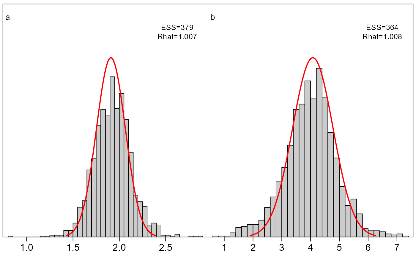
This function plots grid cells of all parameters in a model, comparing the marginal posterior histogram vs the asymptotic normal (red lines) from the inverse Hessian. Its intended use is to quickly gauge differences between frequentist and Bayesian inference on the same model.

If fit$monitor exists the effective sample size (ESS) and R-hat estimates are printed in the top right corner. See https://mc-stan.org/rstan/reference/Rhat.html for more information. Generally Rhat>1.05 or ESS<100 (per chain) suggest inference may be unreliable.

This function is customized to work with multipage PDFs, specifically: pdf('marginals.pdf', onefile=TRUE, width=7,height=5) produces a nice readable file.

Examples

fit <- readRDS(system.file('examples', 'fit.RDS', package='adnuts'))
plot_marginals(fit, pars=1:2)