Plot pairwise parameter posteriors and optionally the MLE points and confidence ellipses.

Usage

# S3 method for class 'adfit'
pairs(
  x,
  pars = NULL,
  order = c("orig", "slow", "fast", "mismatch", "cor"),
  inc_warmup = FALSE,
  diag = c("trace", "acf", "hist"),
  acf.ylim = c(-1, 1),
  ymult = NULL,
  axis.col = gray(0.5),
  label.cex = 0.8,
  limits = NULL,
  add.mle = TRUE,
  add.monitor = TRUE,
  add.inits = FALSE,
  unbounded = FALSE,
  ...
)

Arguments

pars: A character vector of parameters or integers representing which parameters to subset. Useful if the model has a larger number of parameters and you just want to show a few key ones.
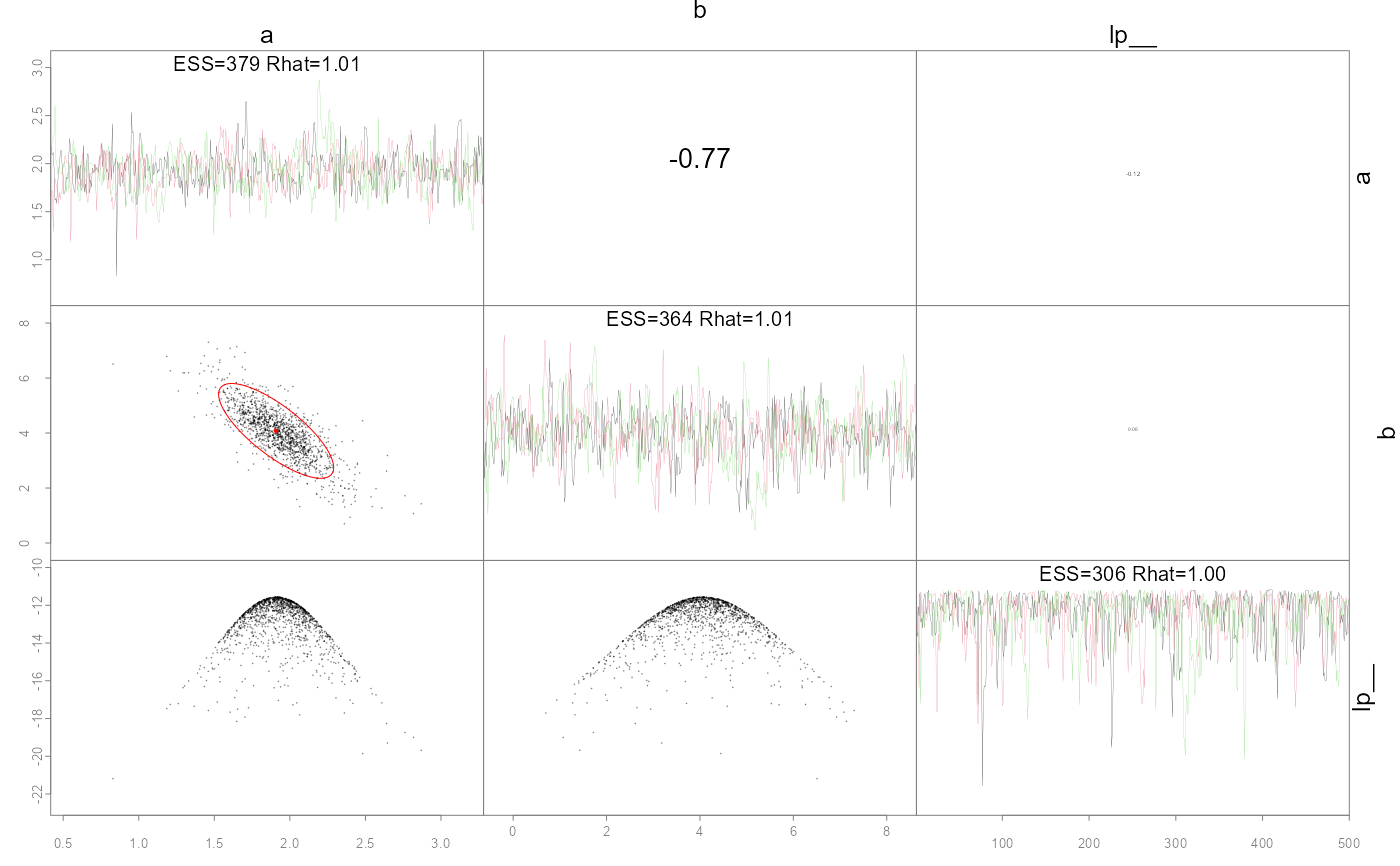
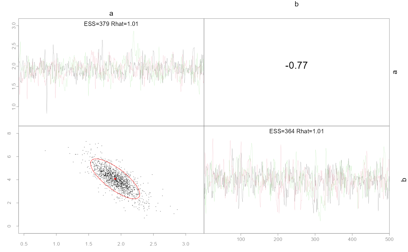
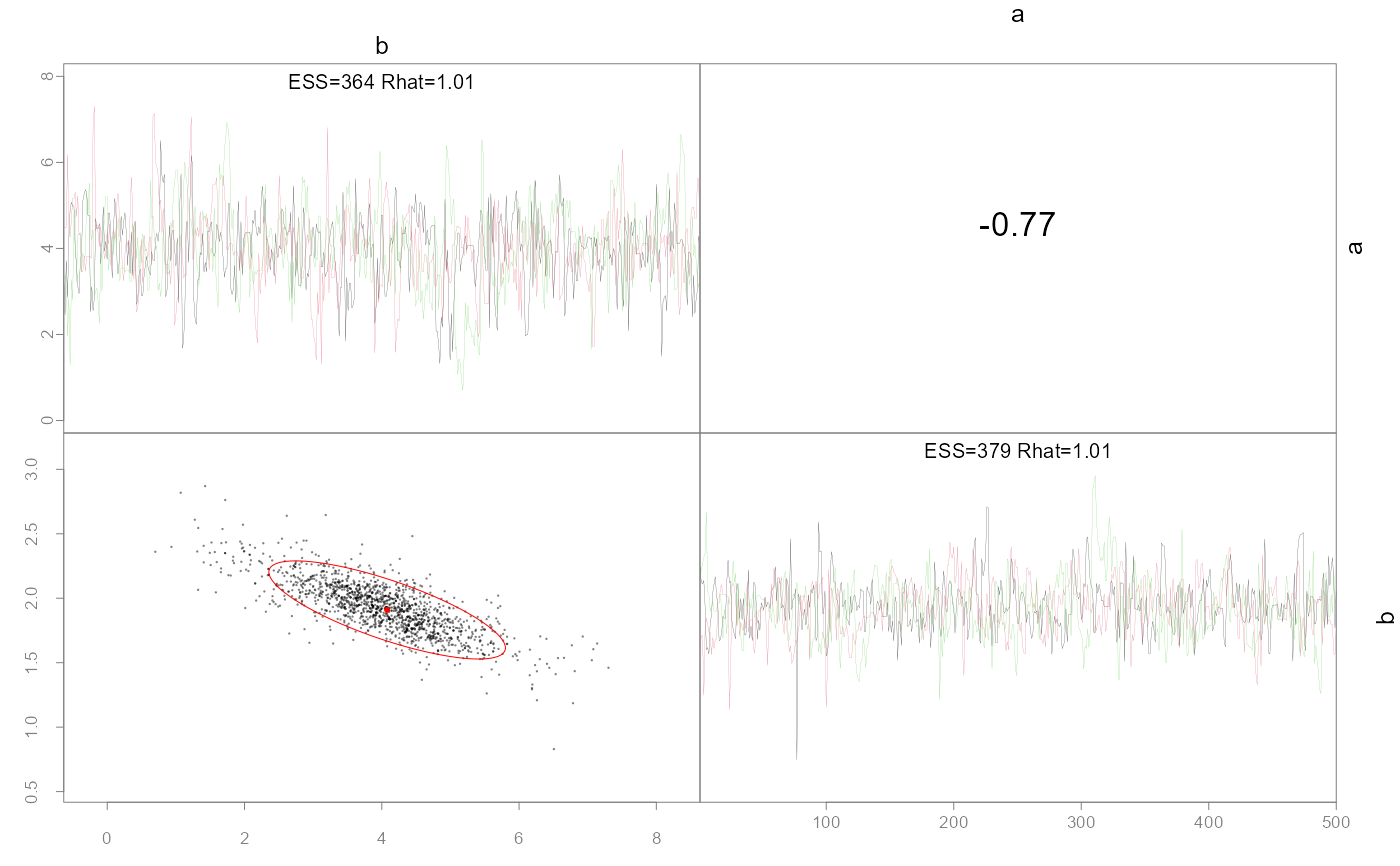
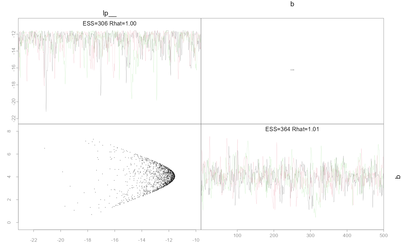
order: The order to consider the parameters. Options are 'orig' (default) to use the order declared in the model, or 'slow' and 'fast' which are based on the effective sample sizes ordered by slowest or fastest mixing respectively. 'mismatch' sorts by parameters with large discrepancies between the MLE and posterior marginal variances, defined as the absolute relative difference of the MLE from the posterior i.e., abs((mle-post)/post). Finally, 'cor' orders by the largest maximum absolute pairwise posterior correlation (including lp__). See example for usage.
inc_warmup: Whether to include the warmup samples or not (default).
diag: What type of plot to include on the diagonal, options are 'acf' which plots the autocorrelation function acf, 'hist' shows marginal posterior histograms, and 'trace' the trace plot.
acf.ylim: If using the acf function on the diagonal, specify the y limit. The default is c(-1,1).
ymult: A vector of length ncol(posterior) specifying how much room to give when using the hist option for the diagonal. For use if the label is blocking part of the plot. The default is 1.3 for all parameters.
axis.col: Color of axes
label.cex: Control size of outer and diagonal labels (default 1)
limits: A list containing the ranges for each parameter to use in plotting.
add.mle: Boolean whether to add 95% confidence ellipses
add.monitor: Boolean whether to print effective sample
add.inits: Boolean whether to add the initial values to the plot
unbounded: Whether to use the bounded or unbounded version of the parameters. size (ESS) and Rhat values on the diagonal.
...: Arguments to be passed to plot call in lower triangular panels (scatterplots).
fit: A list as returned by sample_nuts.

Value

Produces a plot, and returns nothing.

Details

This function is modified from the base pairs code to work specifically with fits from the 'adnuts' package using either the NUTS or RWM MCMC algorithms. If an invertible Hessian was found (in fit$mle) then estimated covariances are available to compare and added automatically (red ellipses). Likewise, a "monitor" object from rstan::monitor is attached as fit$monitor and provides effective sample sizes (ESS) and Rhat values. The ESS are used to potentially order the parameters via argument order, but also printed on the diagonal.

Author

Cole Monnahan

Examples

fit <- readRDS(system.file('examples', 'fit.RDS', package='adnuts'))
pairs(fit)

pairs(fit, pars=1:2)

pairs(fit, pars=c(2,1))

pairs(fit, pars=c('b', 'a'))
pairs(fit, pars=1:2, order='slow')

pairs(fit, pars=1:2, order='fast')

pairs(fit, pars=1:2, order='mismatch')